Thanks to my recently adquired knowledge about how to display stuff on screen with OpenGL, I have implemented in Python an experiment that years ago I wrote in Java: an algorithm that generates images through the NEAT neuroevolutionary method invented in the mid 2000s. When I implemented it in Java, I had to write the NEAT method from zero by reading the scientific papers, because the Java libraries that existed back then didn’t inspire me much confidence. Fortunately, these days and in Python there are a couple solid modules that free me from that responsibility.

I’ll start showing a six minute video that shows some images generated through a few independent evolutionary processes:

A curious phenomenon, although logical, of the results of the programmed neuroevolution mimics what happens in natural evolution: when some pattern appears close to the beginning of the evolutionary run, and for some reason it benefits the genome, the pattern tends to persist for the rest of the evolution in some form or another (for example, the spinal cord).

The experiment works the following way: it generates a population of around 100 genomes that contains the nodes and connections of a neural network. When it gets activated, it will receive two inputs: the x coordinate divided by the width of the resolution the future image will have, and the y coordinate divided by the height of the future image. After the internal calculation, the neural network will produce the four components of a RGBA color: the value for red, for green, for blue, and for the transparency.

When I implemented this experiment for the first time in Java years ago, I programmed it so that each generation’s genome would produce a 32×32 pixels image, that it saved in the hard disk. I had to choose by hand which interested me and add them to a special folder, from which the program would sample to produce the next evolutionary run. However, even then I realized that I was sacrificing vital information so that seeded evolution would work entirely as expected: the genomes hold information about when its nodes and connections appeared for the first time, along with to what species the genomes belong. That information is vital when the genomes reproduce. This time I intended to solve the issue as soon as possible for the Python version, but I ended concluding that I shouldn’t only save the wanted genomes, but all the species involved in that run, along with the generation number. So it made sense to allow the user to save the entire evolutionary state at the chosen stage, all the genomes and the species they belong to. The equivalent to saving the game and reloading it.

The code draws on the screen a 32×32 version of the image each genome produces. In opposition to my previous implementation in Java, in which the genomes got promoted according to how novel they were, now the user has the responsibility to select the genomes he wants to promote. When he decides to move to the next generation, the algorithm scores the genomes in descending order of selection.

I’ve recorded 100 generations of the process in the following video:

The genomes start either completely disconnected or partially connected to the end nodes; I’ve configured it so a possibility of 10% exists so each connection is present at the beginning. That causes some genomes to output no color, or to come out completely black. However, even in the first generation different patterns are already present: vertical bars, diagonals with distorsions, and gradients. It takes just five generations for three genomes to connect with the green output node. However, curiously, it’s only in the 26th generation when a genome connects with the blue output node. A mix of both dominates the evolutionary run, and there’s a complete, or almost complete absence of connections to the red output.

The neural network that the genome converts to must be executed 32 * 32 times (1024 times) only to generate the texture that I’ll display on screen, so it wasn’t feasible during the recording of the video to generate the full images that I include separately in other videos, because the resolution of 1080×1080 implies executing the neural network for each of the selected genomes 1,166,400 times, which takes a while, and for now I haven’t managed to parallelize it (the overhead kills it).

Although the images generated during the recorded evolutionary run didn’t interest me that much, I’ve gathered some of them in the following video:

UPDATE: I’ve managed to parallelize both generating the pixels for all 100 pictures that get displayed on screen for each generation, as well as saving in the background the selected genomes in full. During the last few months I’ve searched for the right parallelization library written in Python, and after considering Pathos for a while, I’ve settled on the brilliant Dask (https://dask.org/), which makes it very transparent.

This is all it takes to map the generation of the pixels for a population and gather the results:

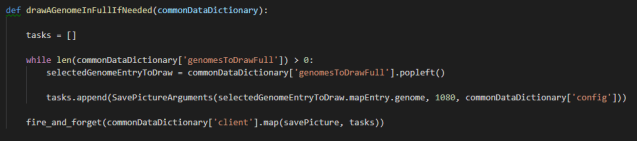
For saving the full pictures, I love the “fire and forget” feature, that allows you to keep advancing the generations while the other cores handle saving the full pictures for the previously selected genomes:

From here I’ll move on to parallelize certain tasks of my main “experiment”, that game thing: running the behavior trees as well as launching the pathfinding queries.